Lagrangian Mechanics - Physics 162

Lagrangian mechanics allows for a generalization of Newton’s laws. As we hinted above, it leads to a more general notion of momentum, which is important for particles moving in electromagnetic fields or through curved spaces. We will also see that it makes the imposition of constraints considerably easier than classic Newtonian mechanics.

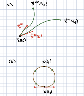
One difference is that, at least in principle, it is not formulated in terms of an initial value problem. Rather, we specify the initial and final positions ${\vec x}_k(t_i), {\vec x}_k(t_f)$ . That you should be able to do this seems reasonable. Given initial positions and velocities you can deduce the final positions, the equations are deterministic, and the amount of data you specify each way is the same. (Actually it is more complicated than that because there can be multiple trajectories with different initial velocities and the same final positions: consider two particles moving in opposite directions on a circle, and bumping into each other later on).

Principle of Stationary Action¶

The basic object in Lagrangian mechanics is...you guessed it...a Lagrangian; this is a function of the positions and velocities of one or several particles:

L = L(x^a_k(t), {\dot x}^a_k(t), t)

(1)

where $a \in \{1,\ldots,d\}$ is the coordinate index for particles in $d$ dimensions (for example, if $d = 3$ we might call $x^1 \equiv x$ , $x^2 \equiv y$ , $x^3 \equiv z$ ), and $k = 1,\ldots,M$ labels different particles. Note that $L$ is a function of $x, {\dot x}$ at a fixed time; thus, even if there is no explicit $t$ -dependence, if $x^a(t)$ is a known trajectory, $L$ depends on $t$ .

Given $L$ , and initial and final times $t_{i,f}$ we can define an action functional (usually called just the action):

S[\{x(t)\}] = \int_{t_i}^{t_f} dt L( x^a_k(t), {\dot x}^a_k(t), t)

(2)

For any trajectory $x^i(t)$ , defined between $t_i$ and $t_f$ , the action is a real number. We call it a “functional” because it can be thought of as a function whose dependent variables are not a collection of discrete numbers, but functions.

The principle of stationary action (sometimes call the “principle of least action”, but this is something of a misnomer). We consider all paths with fixed coordinates at $t_{i,f}$ , defined as

x^a_{k, } = x^a_k(t_i)\ ; \ \ x^a_{k,f} = x^a_k(t_f)

(3)

A “classical trajectory” $x^a_{k,c}$ is one that satisfies the boundary conditions and one for which the action does not change if we make an infinitestimal change of the path. That is, consider two trajectories:

x^a_{k,c}(t)\ ; \ x^a_{k,c}(t) + \epsilon \delta x^a_k

(4)

satisfying the same boundary conditions. This means that $\delta x^a_{k}(t_{i,f}) = 0$ . We take $\eps \ll 1$ to be a small dimensionless parameters. For small enough $\eps$ we can therefore expand

S[\{x^a_{k,c}(t) + \epsilon \delta x^a_k)\}] = S[\{x^a_k(t)\}] + \eps \delta S^{(1)} + \eps^2 \delta S^{(2)} + {\cal O}(\eps^3)

(5)

If $\Delta^{(1)}S[\{x^a_{k,c}\}] = 0$ , then $x^a_{k,c}$ is a classical trajectory.

The Euler-Lagrange equations¶

So far this is all fairly abstract. In fact the principle of stationary action leads to a set of differential equations known as the Euler-Lagrange equations which generalize Newton’s second law. We can write down these equations explicitly in terms of $L$ , by computing $S^{(1)}$ . Let us cary out the expansion explicitly:

\begin{align} S[\{x^a_{k,c}(t) + \epsilon \delta x^a_k)\}] & = S[\{x^a_k(t)\}] + \eps \delta S^{(1)}+ \ldots \\ & = \int_{t_i}^{t_f} dt L(x^a_{k,c}(t) + \epsilon \delta x^a_k, \dot{x}^a_{k,c}(t) + \epsilon \delta \dot{x^a_k}) + {\cal O}(\eps^2)\\ & = S[\{x^a_k(t)\}] + \eps \int_{t_i}^{t_f} \left[ \delta x^a_k \frac{\del L}{\del x^a_k(t)} + \delta {\dot x}^a_k(t) \frac{\del L}{\del \dot{x}^a_k(t)}\right]\big|_{x = x_c} + {\cal O}(\eps^2) \end{align}

(6)

where we are using the Einstein summation notation (see Appendix). Note that $L$ is a standard function of the coordinates and velocities at a fixed time $t$ , so that this makes sense. Now, recall that $\delta \dot{x} = \frac{d}{dt} \delta x$ . Integrating the second term in the last line by parts, we find that

\delta S^{(1)} = \int_{t_i}^{t_f} dt \delta x^a_k \left[ \frac{\del L}{\del x^a_k} - \frac{d}{dt} \frac{\del L}{\del \dot{x}^a_k}\right]\Big|_{x = x_c} + \delta x^a_k \frac{\del L}{\del \dot{x}^a_k} \Big|^{t = t_f}_{t = t_i}

(7)

Now, by the boundary conditions, $\delta x^a_k(t_{i,f}) = 0$ so that the final boundary term vanishes. We have demanded that $\delta S^{(1)}$ vanish for any infinitesimal deformation of $x^a_{k,c}$ , that is for any $\delta x^a_{k,c}$ vanishing at $t_{i,f}$ (at least, if $\eps$ is sufficiently small). Thus, the principle of stationary action is equivalent to the Euler-Lagrange equations:

\frac{\delta S}{\delta x^a_k(t)}\Big|_{x = x_c} \equiv \frac{\del L}{\del x^a_i(t)}(x^a_{k,c}, \dot{x}^a_{k,c}(t)) - \frac{d}{dt} \frac{\del L}{\del \dot{x}^a_i(t)}(x^a\ _{k,c}, \dot{x}^a_{k,c}(t)) = 0

(8)

The first equality defines a functional derivative of $S$ . In the end, all that matters is that this vanishes -- that $S$ does not vary at ${\cal O}(\eps)$ . Classical mechanics does not care whether $S$ is a local or global maximum, local or global minimum, or “saddle point” in which some deformations increase the action at ${\cal O}(\eps^2)$ and oher deformations decrease $S$ .

Without going any further, we can see that this will define $d M$ second order differential equations in time for the $dM$ variables $x^a_k$ .

This formalism naturally includes Newton’s laws. Consider the following Lagrangian for a single particle with mass $m$ in $d$ dimensions:

L = \half m \dot{\vec x} \cdot \dot{\vec x} - V({\vec x})

(9)

Here ${\vec V}\cdot{\vec V} = V^j V^j$ for any vector ${\vec V}$ , where $j$ labels the components. The Euler-Lagrange equations give us:

- \frac{\del V}{\del x^i} - m \frac{d}{dt} \dot{x}^i = 0 \Rightarrow m \ddot{x}^i = - \left(\vec{\nabla} V\right)^i \equiv F^i

(10)

Here ${\vec F} = - \vec{\nabla} V$ is the conservative force associated to the potential $V$ . Note that we have a definite restriction on systems which are well-described by Lagrangian dynamics: many forces are not easily or usefully described in the Lagrangian framework. A classic example is a particle subject to a frictional force linear in velocity:

m \ddot{x} = - \lambda \dot{x} - V'(x)

(11)

(It is not impossible to get this from a variational principle directly in terms of $x$ but this formulation ends up not being especially useful. More insight can be gained by embedding the system in a larger system so that the dynamics of $x$ alone has friction; the energy lost by friction is exchanged with the larger system. But then the dynamics of all of the degrees of freedom can be described by a more conventional if complicated Lagrangian.)

On the other hand, this formalism allows us to generalize away from Newton’s laws in many other directions, including other velocity-dependent forces such as the Lorentz force, and provides new tools for constraining the motion.

Euler-Lagrange equation and generalized coordinates¶

There is a lot more to classical mechanics than just the motion of a collection of point particles in Euclidean space. Other systems include:

The motion of the orientational degrees of freedom of a rigid body such as a top or a satellite.
The dynamics of some elastic system such as a rubber sheet or even a piece of metal.
Continuum fields such as the electromagnetic or gravitational fields

All of these can be described within the framework of Lagrangian mechanics.

In general we start with a set of generalize coordinates $q^I$ . These could be the position variables $x^a_k$ for particles in Euclidean space, or anyo of the above examples. If we have a Lagrangian $L(q^I, {\dot q}^I, t)$ , and an action

S[\{q^I(t)\}] = \int_{t_i}^{t_f} dt L(q^I, {\dot q}^I, t)

(12)

The Euler-Lagrange equations are

\frac{\del L}{\del q^I} - \frac{d}{dt} \frac{\del L}{\del \dot{q}^I} = 0

(13)

If we define the generalized momentum as

p_I(q^I, \dot{q}^I) = \frac{\del L}{\del\dot{q}^I}

(14)

and the generalized force as

{\cal F}_I(q^I, \dot{q}^I) = \frac{\del L}{\del q^I}

(15)

then the Euler-Lagrange equations can be written as

\frac{d}{dt} p_I = {\cal F}_I

(16)

which clearly takes the form of Newton’s second law.

All of this discussion has been fairly abstract, so let us study an example.

Particle in a magnetic field¶

Alternatively we consider the case where we have standard coordinates but a nontrivial generalized momentum. That is, consider a particle with mass $m$ and charge $e$ in a static magnetic field $\vec{B}$ . Maxwell’s equations (assuming no magnetic monoploes; we haven’t observed them at any rate) imply that $\vec{\nabla} \cdot \vec{B} =$ , which means that in Euclidean space without any holes we can use the Poincar'e theorem to write

\vec{B} = \vec{\nabla} \times \vec {A}

(17)

for some $\vec{A}$ . I claim the correct Lagrangian for a particle in this field is:

L = \half m \dot{\vec{x}}^2 + \frac{e}{c} \dot{\vec{x}} \cdot \vec{A}(x)

(18)

The generalized momentum is

p_i = \frac{\del L}{\del \dot{x}^i} = m \dot{x}^i + \frac{e}{c} A^i

(19)

and the generalized force is

{\cal F}^i = \frac{\del L}{\del x^i} = \frac{e}{c} \dot{x}^j \del_i A^j

(20)

The Euler-Lagrange equations become

\begin{align} \frac{d p^i}{dt} & = m \ddot{x}^i + \frac{e}{c} \dot{x}^j \del_j A^i\\ & = {\cal F} \\ & = \frac{e}{c} \dot{x}^j \del_i A^j \end{align}

(21)

so that

\begin{align} m \ddot x^i & = \frac{e}{c} {\dot x}^j (\del_i A^j - \del_j A^i)\\ & = \frac{e}{c} {\dot x}^j \epsilon_{ijk} (\vec{\nabla}\times {\vec A})^k\\ & = \frac{e}{c} {\dot x}^j \epsilon_{ijk} B^k \\ & = \frac{e}{c} (\dot{\vec{x}}\times\vec{B})^i \end{align}

(22)

which is the Lorentz force law.

Note that the final equations of motion depend on the magnetic field $B$ and not on the vector potential $A$ . People often assume that the physical fields are the electromagnetic fields, and $A$ is not unquely determined since the “gauge transformation”

\vec{A} \to \vec{A} + \vec{\nabla} \Lambda

(23)

does not change $E$ or $B$ . The generalized momentum does depend explicitly on ${\cal A}$ , and so in this case is not invariant under gauge transformations.

Counter-example: frictional motion¶

The question of friction came up in class. In general this does not have a straightforward Lagrangian description. Let us explore this a little.

Linear friction without an external force¶

Consider the case of linear velocities:

m \ddot{q} = - \lambda {\dot q}

(24)

We will work in one dimension though the same techniques wiull work in higher dimensions. The above is standard friction if $\lambda > 0$ . (If $\lambda < 0$ then the force increases with velocity and we get runaway behavior. You can see this by explicitly solving the above equation).

Now let us try to find $L(q,{\dot q})$ which produces this. We need

\frac{d}{dt} \frac{\del L}{\del {\dot q}} = \frac{\del L}{\del q}

(25)

Clearly to get the $m{\ddot q}$ term we need $L = \half m {\dot q}^2$ . Getting a term linear in voleicty is another story. It must take the term ${\dot q} f(q)$ for rither the generalized force or the generalized momentum to produce such a term. But this is automatically a total derivative: we can always find an $F(q)$ such that $F'(q) = f(q)$ ; then ${\dot q} f(q) = \frac{d}{dt} F(q)$ . This is a total derivative that will not contribute to the Euler-Lagrange equations, as you can see by adding this term.

One out is to allow the Lagrangian to be time-dependent:

L = \half e^{2 \lambda t/m} m {\dot q}^2

(26)

If we plug this into the action, though, we can see that we get the standard action if we change the time coordinate to $\tau = \tau_0 e^{-2\lambda t/m}$ . In fact if you apply this change to the eqautions of motion for a frictional particle, you get back the standard equations of motion. One-dimensional motion is somewhat special.

One can instead consider the following Lagrangian:

S = \int dt \beta(t) (m \ddot{q} + \lambda \dot{q}) = \int dt \left(-m \dot \beta {\dot q} + \lambda \beta {\dot q}\right)

(27)

where in the second term we have integrated by parts and ignored boundary terms. Here we consider $q,\beta$ as dynamical variables and it should be clear that the variational principle yields both the frictional equation of motion (from teh Euler-Lagrange equation for $\beta$ ) as well as for $\beta$ . From this we get the following equations of motion:

\begin{align} m \ddot{q} & = - \lambda \dot{q} \\ m \ddot{\beta} & = \lambda \dot{\beta} \end{align}

(28)

So here we can see that this “auxiliary” field $\beta$ , which we introduced as a Lagrange multiplier, has a runaway term: $\

Lagrangians and coordinate changes¶

General statement¶

Consider a change of coordinates from $x^a_k$ to $q^{I = 1,\ldots Md}$ . In this case we can write

:label: change_coords_lag L(x, \dot{x}) = L(x(q), \dot{x}(q,\dot q)) = \tilde{L}(q, \dot{q})

(29)

where

\dot{x}^a_k = \dot{q}^I \frac{\del x^a_k}{\del q^I}

(30)

We claim that the Euler-Lagrange equations for $x^a_k$ derived from $L$ and the Euler-Lagrange equations for $q^I$ derived from ${\tilde L}$ are in fact equivalent. That is,

\frac{\del L}{\del x^a_k} - \frac{d}{dt} \frac{\del L}{\del\dot{x}^a_k} = 0 \Leftrightarrow \frac{\del {\tilde L}}{\del q^I} - \frac{d}{dt} \frac{\del {\tilde L}}{\del \dot{q}^I} = 0

(31)

The point is that you can perform your coordinate transformations at the level of the Lagrangian, and then compute the Euler-Lagrange equations in the new coordinates, which is often easier than computing the change of variables at the level of the equations of motion.

To start with, the partial derivatives in (30)

{\cal M}(ak\ ; I) = \frac{\del x^a_k}{\del q^I}

(32)

can be thought of as an $dM \times dM$ matrix at a given value of $q^I$ ; this is the “Jacobian” of the coordinate transformation between $x$ and $q$ , and it is an invertible matrix if the coordinate transformation is itself non-singular (is a good coordinate transformation). In particular, we can define the inverse Jacobian as

{\cal M}^{-1}(I\ ; ak)

(33)

By the chain rule,

{\cal M}(I'\; ak) {\cal M}(ak, I) = \frac{\del q^{I'}}{\del x^a_k} \frac{\del x^a_k}{q^I} = \frac{\del q^{I'}}{\del q^I} = \delta^I_{I'}

(34)

where $\delta^I_{I'}$ is the Kronecker delta symbol (see the Appendix for a definition). We can similarly show that

{\cal M}(ak\; I) {\cal M}^{-1}(I\; a'k') = \delta^a_{a'} \delta^k_{k'}

(35)

To see why invertability is important let us think of the canse of $dM = 1$ . Then the matrix is just ${\cal M} = \frac{\del x}{\del q}$ . Consider a particular point $q_0$ about which we wish to study the coordinate transformation. the value of $x$ is $x_0 = x(q_0)$ . At an infinitesimal distance $\delta q$ away from $q_0$ , we have

x(q_0 + \delta q) = x_0 + \frac{\del x}{\del q} \delta q + {\cal O}(\delta q^2)

(36)

Now the inverse of $\frac{\del x}{\del q}$ is just $\left(\frac{\del x}{\del q}\right)^{-1}$ , so ${\cal M}$ fails to be invertible if it is zero. If it is zero at $q_0$ the $x = x_0 + {\cal O}(\delta q^2)$ . In ither words, at leading order in $\delta q$ , $x$ does not change and at this order the coordinate change from $q \to x$ is a many-to-one map. For the rest of this section we will assume the coordinate transformation is invertible but there are many cases where it fails to be at least at a point: a good example is the transformation from Catrtesian to polar coordinates in $d = 2$ , for which the origin is a singular point.

Now,

\begin{align} p_I & = \frac{\partial {\tilde L}}{\partial \dot{q}^I}\\ & = \frac{\del}{\del \dot{q}^I} L(x(q), {\cal M}(ak; I) \dot{q}^I)\\ & = {\cal M}(ak\ ; I) p^a_k \end{align}

(37)

while

\begin{align} {\cal F}_I & = \frac{\del}{\del q^I} L(x(q), {\cal M}(ak\ ; I) \dot{q}^I) \\ & = {\cal M}(ak\ ; I) {\cal F}^a_k + \frac{\del {\cal M}(ak\ ; J)}{\del q^I} \dot{q}^J p^a_k \end{align}

(38)

The Euler-Lagrange equations we derive from ${\tilde L}$ for $q^I$ are:

\begin{align} \frac{d}{dt} p_I - {\cal F}_I & = \frac{d}{dt} \left(\frac{\del x^a_k}{\del q^I} p_a^k\right) - \frac{\del x^a_k}{\del q^I} {\cal F}^a_k - \frac{\del^2 x^a_k}{\del q^I \del q^J} \dot{q}^J p^a_k \\ & = \frac{\del x^a_k}{\del q^I}\left({\dot p}^a_k - {\cal F}^a_k\right) + \frac{\del^2 x^a_k}{\del q^J \del q^I} \dot{q}^J p_a^k - \frac{\del^2 x^a_k}{\del q^I \del q^J} \dot{q}^J p^a_k \\ & = {\cal M}(ak\ ; I) \left(\dot{p}^a_k - {\cal F}^a_k\right) \end{align}

(39)

The second line follows from applying Leibniz’s rule to the time derivative of ${\cal M} p$ . The last line is an invertible matrix times the Euler-Lagrange equations for $x^a_k$ derived from $L$ . Thus the two forms of the Euler-Lagrange equations are equivalent; one vanishes if and only if the other does (assuming the coordinate transformation is invertible).

Example: changing to polar coordinates¶

Consider a single particle in two dimensions with the Lagrangian

L = \half m (\dot{x}^2 + \dot{y}^2) - V(r = \sqrt{x^2 + y^2})

(40)

The Euler-Lagrange equations are:

\begin{align} m \ddot{x} & = - \del_x V = - \frac{x}{r} V'(r)\\ m \ddot{y} & = = \del_y V = - \frac{y}{r} V'(r)\\ \end{align}

(41)

We can consider instead polar coordinates $(r,\phi)$ , defined by:

x = r \cos\phi\ , \ \ y = r \sin \phi

(42)

To change to equations in polar coordinates, we find:

\ddot{x} = \ddot{r}\cos\phi - 2 \dot{r} \dot{\phi} \sin\phi - r \ddot\phi\cos\phi

(43)

and similarly for $y$ . On the other hand, we can quickly show that

L = \half m \left(\dot{r}^2 + r^2 \dot{\phi}^2\right) - V(r)

(44)

where I have tropped the tilde. Note that $r\dot{\phi}$ is the physical velocity in the ${\hat \phi}$ direction, and $\dot{r}$ is of course the radial velocity $v^{\phi}

We can first compute the generalized momentum

\begin{align} p_r & = \frac{\del L}{\del \dot{r}} = m \dot{r}\\ p_{\phi} & = \frac{\del L}{\del\dot{\phi}} = m r^2 \dot \phi = m r v^{\phi} = \ell \end{align}

(45)

The point is that the generalized momentum $p_{\phi}$ can be identified with the alngular momentum $\ell$ about the origin $r = 0$ . The Euler-Lagrange equations are:

\begin{align} m \ddot{r} & = - \del_r V\\ \frac{d}{dt} m r^2 \phi & = \frac{d}{dt} \ell = 0 \end{align}

(46)

which you can also show are the equations of motion by applying the transformation from Euclidean to polar coordinates to the Euler-Lagrange equations for $x,y$ . Note that $V = V(r)$ inplies that there is no generalized force associated to the generalized momentum or angular momentum $\ell$ ; in other words, there is no torque. There would be torque (aka a generalized force in the angular direction) if $V$ had any $\phi$ -dependence in it. The relationship between the independence of $L$ of certain coordinates, and a conservation law such as the conservation of angular momentum, is a general story we will return to below.