Two-state systems as phenomenological models

Here we are going to consider the low-energy dynamics of generally complicated systems. While we have not gone into length in talking about time-dependent probes yet, you can intuit that interacting with a given system will generally involve adding or subtracting energy. For example, usually an experiment is a time-dependent process, so right there you know that energy will not be conserved. But by the energy-time uncertainty principle, if you interact sufficiently slowly, the energy input will not be large. Thus, if the systems starts in the ground state or first excited state, and the energy input is small compared to the energy difference between the first and second excited state, you can assume that before and after the experiment is done, it will remain in some superposition of teh ground state and first excited state. The Hilbert space is thus quite simple, and the Hamiltonian will be parameterized by just a few numbers (the entries of a $2\times 2$ Hermitian matrix) which one can fit to experiments, in the case that first--principles calculations are too hard.

Double-well potential¶

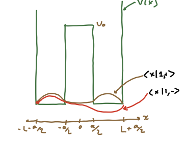
The first system we will examine is one that we could in principle solve exactly. Consider the following double-well potential for a 1d particle with mass $m$:

Thus $L$ is the width of each well, and $a$ the width of the barrier.

Warmup: Infinite barrier¶

To get some intuition for this we will start with the $V_0 \to \infty$ case. In this case, we take $\cH_{L,R}$ to be the Hilbert space for the particle in the left or right wells, and $\cH_{\infty} = \cH_{L} \oplus \cH_{R}$. The particle can sit in either the left well or the right well, and the Hamiltonian is diagonal. The wavefunctions and eigenenergies are:

So each energy level is doubly degenerate, as the energy levels for the particle localized in the left or the right well are the same (since the wells have the same width and boundary conditions). Note that we can write these wavefunctions as

where $A$ is an index labeling the wells.

In this case, parity is a clear symmetry of the theory. As we have already discussed, we can re-arrange the energy spectrum in terms of parity eigenstates:

Large but finite barrier¶

If we let $V_0$ be finite, the degeneracy is split as is generically the case in 1d problems. We can expect that the splitting goes to zero as $V_0 \to \infty$ and remains very small for $E \ll V_0$, since the barrier will look close to infinite. What we do know is that the energy eigenstates will be parity eigenstates.

A hand-waving argument is that the splitting scales like

The prefactor is based on a classical velocity $v$ such that $\half m v^2 = E$ and we have used the ground state energy for $E$; $L/v$ is proportional to the rate the particle his the barrier as is bounces back and forth in the well. That is the hand-waving part. The exponential prefactor can be calculated exactly or via the WKB approximation which we will discuss later. But we can start to see where it comes from: for $E < V_0$, the wavefunction in the barrier region $|x| \leq \frac{a}{2}$ is:

where

The precise value of $A, B$ come from matching to the wavefunctions in the classically allowed ($V = 0$) regions.

Sketches of the two lowest-energy states, which are deformations of the ground states for finite $V_0$, are shown below.

For any $\ket{n,\pm}$ with $E_n \ll V_0$, the story is similar. At infinite $V_0$, the states are symmatric and antisymmetric combinations of the energy states in each of the two wells. For finite_V_0$ the states are close to this, with the wavefunction small but finite under the barrier. We can deduce that this will introduce no nodes for the symmetric case but introduce an additional node for the antisymmetric case. Since the energy eigenstates increase with the number of nodes, the antisymmetric wavefunction will have slightly higher energy than the symmetric wavefunction. The spectrum will deform as shown below.

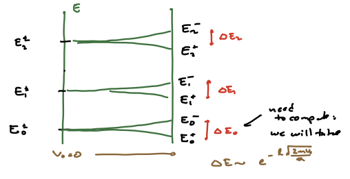
Let us stick to the lowest-energy states, which we will call $\ket{\pm}$. These will have energies $E_{av} \pm \half \Delta E$ where $E_{av}, \Delta E$ are functions of $V_0, a, L$. As illustrated in the figure below, we can form lineaer combinations

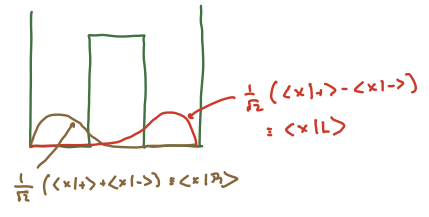
Note that we do not get preciselocalization in one well or the other -- that would require all $\ket{n,\pm}$ (this is not meant to be an obvious statement, but it is worth thinking about).

Now let us start with the particle localized in the left well, by which we mean

Evolving this in time, we find

If we call the probability of the particle being found in the right well $p_R = |\brket{R}{\psi(t)}$, a little algebra gives us

The interpretation is that a low-energy particle initially confined to one well will tunnel to the other well. This is a classically forbidden process. When the energy is well below the barrier, we define the tunneling time as the time for the particle state to evolve to $\ket{R}$:

This is exponentially small in $a\sqrt{2m V_0}/\hbar$, as discussed above. The exponential suppression $\sim e^{-S/\hbar}$ for some $S$ is characteristic of quantum tunneling processes.

The Hamiltonian in the energy/parity eigenstate basis in which $\ket{+}$ is represented by $\begin{pmatrix} 1 \\ 0 \end{pmatrix}$ and $\ket{-}$ is represented by $\begin{pmatrix} 0 \\ 1 \end{pmatrix}$ is:

Working in the position basis in which $\ket{L}$ is represented by $\begin{pmatrix} 1 \\ 0 \end{pmatrix}$ and $\ket{R}$ is represented by $\begin{pmatrix} 0 \\ 1 \end{pmatrix}$, we have:

We can think of this off-diagonal term as a ``hopping" term that drives transitions between $\ket{L}$ and $\ket{R}$; the transition rate, after all, scales with $\Delta E$.

In fact you can very quickly show this is the most general Hermitian operator that commutes with the matrix

which exchanges $\ket{L}$ and $\ket{R}$.

Asymmetric double well potential¶

Next we will consider an asymmetric double well, with a potential as sketched below

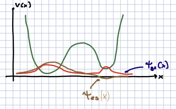
We are not going to worry too much about the details of the potential but argue for a simple model for the lowest-energy states.

Near each local minimum, which we label by $x_L, x_R$, we can define $m \omega_{L,R}^2 = V''(x_{L,r})$. To first approximation, when the barrier between them is sufficiently high and wide, we expect sufficiently low-energy states to be harmonic oscillator states localized near $x_L$ with energies $V(x_L) + \hbar \omega_L(n_L + \half)$, and low-energy states localized near $x_R$ with energies $V(x_R) + \hbar \omega_R(n_R + \half)$. These get distorted by tunneling through the barrier. We assume that $V(x_L) - V(x_R) + \half \hbar(\omega_L - \omega_R)$ is small compared to $\hbar\omega_{L,R}$, and that the tunneling rate $\Gamma$ is much smaller than $\omega_{L,R}$. Then it is reasonable to expect that the two lowest-energy states are linear combinations of the approximate SHO ground state wavefunctions localized near $x_{L,R}$. If $V(x)$ is almost symmetric, we might expect the ground state and first excited states to the the wavefunctions $\psi_{gs}, \psi_{es}$ shown in the figure above.

Since we no longer have any symmetry, the Hamiltonian in the basis of states localized near either $x_L$ or $x_R$ is the most general Hermitian matrix:

With some work you can show that with a suitable phase change in the basis vector for the left-localized state

yields the above Hamiltonian with $\gamma = 0$. The matrix elements $E_{1,2}, \Delta E$ can be fit to experiment (up to an overall shift in the diagonal matrix elements).

Molecular models¶

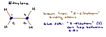
Volume 3 of the Feynman lectures contain a nice discussion of low-energy models for electrons in a molecule. We will briefly discuss the simplest example, to give the discussion above a slightly more real-world flavor. The figure below shows a simple schamtic diagram of an ethylene molecule, consisting of four Hydrogen atoms attached to a pair of Carbon atoms. The lines are the atomic bonds. This system has two “$\pi$-electrons” which can hop between the two carbon atoms. We assume the electrons do not interact and that their spin degrees of freedom render them effectively distinguishable (we will discuss distinguishable vs. indistinguishable particles at some point in 162b). For each of them, then, the Hilbert space is two-dimensional. Note that flipping the molecule right to left does not change the appearance of the molecule. So we have the parity symmetry that we also made use of in the case of the symmetric rectangular double well. Following the discussions above, e can write the Hamiltonian in the basis of positions (which carbon atom the electron is bound to as):

where $E_0, A$ are real parameters. It is easy to see the energy eigenstates are symmetric and antisymmetric combinations of the localized states; these have energies $E_{\pm} E_0 \mp \Delta E$, and $\hbar/\Delta E$ is the time scale over which electrons hop between the Carbon atoms. The essential point is that given symmetry argumenst and some broad-brush understanding of the dynamics we can deduce the form of teh Hamiltonian; the parameters can then be fit to experiment.