Orbital Angular Momentum

Representations of angular momentum operators

Let us consider particles with no intrinsic spin. (Except for the Higgs boson, these will typically be composite particles such as atoms whose total spin vanishes, where we treat the atoms as point particles. Anothe rexample is the \(\alpha\)-particle which is a helium-4 nucleus, a spin-\(0\) bound state of 2 protons and 2 neutrons.) If the particles are moving in \(\mathbb{R}^3\), their Hilbert space is \(L^2(\CR^3)\), and rotations act nontrivially. We can define the action of rotations in the position basis:

\[U(R)\ket{\vec x} = \ket{\vec{R x}}\]

where \(R\) is the \(3\times 3\) matrix acting on vectors in \(\CR^3\). Note that this means that

\[\bra{x} U(R) = \bra{x} U^{\dagger}(R^{-1}) = \bra{(R^{-1} x}\]

Thus, if we let \(\ket{\psi'} = U(R) \ket{\psi}\),

\[\psi'(x) = \brket{x}{\psi'} = \bra{x} U(R)\ket{\psi} = \brket{R^{-1} x}{\psi} = \psi(R^{-1}x)\]

Let us conisder infinitesimal rotations by an angle \(\theta\) about the \(z\) axis, for which

Then

\[\begin{split}\begin{align} \psi'(x) & = \psi(x + \theta y, y - \theta x, z) = \psi(x) + \theta y\frac{\del}{\del x} \psi - \theta x \frac{\del}{\del y} \psi\\ & = {\bf 1} - \frac{i\theta}{\hbar} (J_z \psi)(x) \end{align}\end{split}\]

Since \(\frac{\del}{\del x^i} = \frac{i}{\hbar} p_i\), we have

\[J_z = {\hat x} {\hat p}_y - {\hat y} {\hat p}_x\]

Similar arguments yield

\[\begin{split}\begin{align} J_x & = {\hat y} {\hat p}_z - {\hat z}{\hat p}_y \\ J_y & = {\hat z} {\hat p}_x - {\hat x}{\hat p}_z \end{align}\end{split}\]

or

\[{\vec J} = {\hat{\vec x}} \times {\hat{\vec p}}\]

If we replaced the operators by classical observables, there would just be the classical angular momenta. We can check that, acting on states, these have the correct commutation relations \([J_I, J_J] = i \hbar \epsilon_{IJK} J^K\).

It is natural to express the angular momentum operators as derivative operators in spherical coordinates \((r,\theta,\phi)\), since rotations fix \(r\). Recalling the transformations:

\[\begin{split}\begin{align} x & = r\sin\theta\cos\phi\\ y & = r\sin\theta\sin\phi\\ z & = r\cos\theta \end{align}\end{split}\]

with some labor we can work out the angular momentum operators. Note that by convention, the differential operators are called \(L_i\) instead of \(J_i\):

\[\begin{split}\begin{align} L_z & = \frac{\hbar}{i} \frac{\del}{\del\phi}\\ L_{\pm} & = i\hbar e^{\pm i \phi} \left(\cot\theta \frac{\del}{\del\phi} \mp i \frac{\del}{\del\theta}\right)\\ {\vec L}^2 & = - \left[\frac{1}{\sin\theta}\frac{\del}{\del\theta}\left(\sin\theta \frac{\del}{\del\theta}\right) + \frac{1}{\sin^2 \theta}\frac{\del^2}{\del\phi^2}\right] \end{align}\end{split}\]

It is worth noting that \({\vec L}^2\) appears in the Laplacian in spherical coordinates and in fact contains all of the angular derivatives:

\[{\vec\nabla}^2 = \frac{1}{r} \frac{\del^2}{\del r^2} r - \frac{{\vec L}^2}{r^2}\]

Spherical harmonics

In spherical coordinates, the orbital angular momentum operators act on the angular coordinates. We expect that when we write angular momentum eigenstates \(\ket{\alpha,\ell, m}\) (where \(\alpha\) denotes additional degrees of freedom, perhaps tied to the behavior of the wavefunction in the radial direction), the wavefunctions will take the form

\[\brket{r\theta\phi}{\alpha\ell m} = f_{\alpha}(r) Y_{\ell,m}(\theta,\phi)\]

Alternatively we might have particles constrained to live on a sphere, for which \(Y_{\ell,m}\) then become a complete basis of functions on \(S^2\). The \(Y_{\ell,m}\) are known as spherical harmonics.

We can quickly deduce the \(\phi\)-dependence:

\[L_z Y_{\ell,m}(\theta,\phi) = \frac{\hbar}{i} \frac{\del}{\del \phi} Y_{\ell,m}(\theta,\phi) = \hbar m Y_{\ell,m}(\theta,\phi)\]

which means

\[Y_{\ell,m}(\theta,\phi) = e^{i m \phi} f_{\ell,m}(\theta)\]

To go further, we can start by solving the first order differential equation

\[L_- Y_{\ell,-\ell}(\theta,\phi) = - \hbar e^{-i\ell\phi}\left[ \frac{\del}{\del\theta} - \ell \cot\theta\right] f_{\ell,m}(\theta) = 0\]

This is solved if \(f_{\ell,m} = A \sin^{\ell}(\theta)\). After properly normalizing \(Y_{\ell,-\ell} = A e^{-i\ell \phi} \sin^{\ell}\theta\), we can construct the other functions \(Y_{\ell,m}\) with applications of \(L_+\).

The general solution is

\[Y_{\ell,m}(\theta,\phi) = (-1)^m \sqrt{\frac{2\ell + 1}{4\pi} \frac{(\ell - m)!}{(\ell + m)!}} e^{i m\phi} P_{\ell}^m(\cos\theta)\]

where \(P_{\ell}^m(x)\) are the associated Legendre functions. These can be looked up in a good quantum mechanics textbook, or in a book of special functions such as this one (now online). The spherical harmonics form an orthonomal basis of functions on the sphere; thus

\[\int_0^{2\pi} d\phi \int_0^{\pi} \sin\theta d\theta Y^*_{\ell,m}(\theta,\phi)Y_{\ell',m'}(\theta,\phi) = \delta_{\ell,\ell'}\delta_{m,m'}\]

Example: rigid rotor

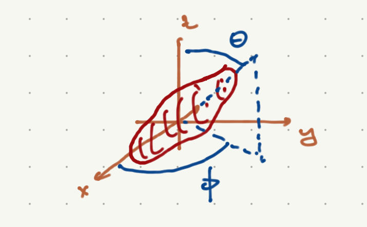
We can consider the following model of the rotational states of an axisymmetric molecule in its center of mass frame, as pictured below.

A molecule rotating about the center of mass

Classically, the rotational kinetic energy is taken to be

\[H = \frac{{\vec L}^2}{2I}\]

where \(I\) is the moment of inertia of the rotor. We can also simply demand that the Hamiltonian be invariant under rotations about the center of mass. This means that there is no potential energy as a function of \(\theta,\phi\); the only operators available are functions of \({\vec L}^2\). If we are looking at sufficiently small values of teh angular momenta, we can expand the Hamiltonian in powers of \({\vec L}^2\) and then the leading order term will be that above.

The energy levels are therefore \(E_{\ell} = \frac{\hbar^2 \ell(\ell + 1)}{2I}\) with degeneracy \((2\ell + 1)\). A basis of states is then \(\ket{\ell,m}\), with \(\brket{\theta,\phi}{\ell,m} = Y_{\ell,m}(\theta,\phi)\).

This degeneracy could be split simply by an additional term \(\delta H = \gamma L_z\), for example. This could arise if the molecule had an unenev distribution of charge so that its rotation induces a current and thus a magnetic moment. In the presence of a magnetic field \(B_z\), we would then induce such a coupling of the form \(\delta H = - \mu B)z L_z\). The wavefunctions \(Y_{\ell,m}\) are still eigenstates of the full Hamiltonian, but the energies are now

\[E_{\ell,m} = \frac{\hbar^2 \ell(\ell + 1)}{2I} - \mu B_z \hbar m\]

and the spectrum is completely nondegenerate in general (if B is large enough, there are special values of \(B_z\) where states with different values of \(\ell\) start to overlap because of the large splitting.)