Representations of the rotation group

General structure

We will find that the commutation relations of infinitesimal operators put strong constraints o n the irreducible representations of the rotation group. The basic strategy is somewhat analogous to that we used to solve for the simple harmonic oscillator.

Recall that for infinitesimal rotations by angle \(\theta\) about an axis described by unit vector \({\hat n}\), \(R \sim \delta - i \theta \frac{{\vec J}\cdot{\hat n}}{\hbar}\); the commutation relations of \(J\) are: \([J_I, J_J] = i\hbar \epsilon_{IJK} J^K\).

In a unitary representation, \(U(R) \sim {\bf 1} - i \theta \frac{{\hat J}^I {\hat n}_I}{\hbar}\) where \({\hat J}\) is a Hermitian operator. As we have shown, the commutation relations of infinitesimal operators determine the structure of non-Abelian multiplication for any group elements (which can be built from successive infinitesimal rotations). Therefore \({\hat J}^I\) must satisfy the same algebra as the matrices we constructed above: \([{\hat J}_I, {\hat J}_J] = i \hbar \epsilon_{IJK} {\hat J}^K\). Following the discussion in the previous section, the action of a finite rotation by angle \(\theta\) about an axis \({\hat n}\) is then:

\[U(R(\theta,{\hat n})) = e^{- i \theta {\hat n}\cdot{\hat{\vec J}}/\hbar}\]

We start by finding a set of commuting Hermitian operators built from \({\hat{\vec J}}\). These can be mutually diagonalizable. First, you can show that \({\vec J}^2\) commutes with all of \({\hat J}_I\). You can show this by brute force. You can also note that \({\vec J}\) generates infinitesimal rotations; but \({\vec J}^2\) is the square of a vector and isn’t exopected to change under rotations. In saying this I am sweeping a lot under the rug – what is a vector operator and how does it transform?.

Since \({\vec J}^2\) commutes with \(J_I\) for all \(I\), the eigenvalue for \({\vec J}^2\) is invariant under rotations. Since the definition of an irreducible representation is that the only subspace which is invariant under rotations is the whole vector space, an irrep must have a fixed value of \({\vec J}^2\).

By tradition we also pick the operator \({\hat J}_z\) and mutually diagonalize \({\vec J}^2\), \(J_z\). That is the irrep should have an orthornormal basis \(\ket{\alpha,\beta}\) such that \({\vec J}^2\ket{\alpha,\beta} = \alpha \ket{\alpha,\beta}\) and \({\hat J}_z\ket{\alpha,\beta} = \beta\ket{\alpha,\beta}\).

Next, we construct the operators

\[J_{\pm} = J_x \pm i J_y = J_{\mp}^{\dagger}\]

These satisfy the commutation relations:

\[\begin{split}\begin{align} [J_z, J_{\pm}] & = \pm \hbar J_{\pm} \\ [J_+,J_-] & = 2\hbar J_z\\ [J_{\pm}, {\vec J}^2] & = 0 \end{align}\end{split}\]

First, we can show that \(\alpha \geq \beta^2\). This is based on the relations:

\[{\vec J}^2 - J_z^2 = J_x^2 J_y^2 = J_+ J_- + J_- J_+\]

Thus

\[\begin{split}\begin{align} \alpha - \beta^2 & = \bra{\alpha,\beta} ({\vec J}^2 - J_z^2) \ket{\alpha,\beta}\\ & = \bra{\alpha,\beta} (J_+ J_- + J_- J_+) \ket{\alpha,\beta}\\ & = ||J_- \ket{\alpha,\beta}||^2 + || J_+ \ket{\alpha,\beta}||^2 \geq 0 \end{align}\end{split}\]

Next, from the commutation relations for \(J_{\pm}, J_z\), we find

\[ J_{\pm}\ket{\alpha,\beta} = C_{\pm} \ket{\alpha,\beta \pm \hbar}\]

where \(C_{\pm} \in \CC\) is a constant. Given this, \(\beta\) will have a maximum \(\beta_{max}^2 \leq \alpha\) and a minimum \(\beta_{min}^2 \leq \alpha\) such that

\[\begin{split}\begin{align} J_+ \ket{\alpha,\beta_{max}} & = 0\\ J_-\ket{\alpha,\beta_{min}} & = 0 \end{align}\end{split}\]

Now, we can use the commutation relations to find:

\[J_{\pm} J_{\mp} = J_x^2 + J_y^2 \mp [J_x,J_y] = {\vec J}^2 - J_z^2 \pm \hbar J_z\]

Therefore:

(312)\[\begin{split}\begin{align} J_+ J_- \ket{\alpha,\beta_{min}} & = 0 = \alpha - \beta_{min}^2 + \hbar \beta_{min}\\ J_- J_+ \ket{\alpha,\beta_{max}} & = 0 = \alpha - \beta_{max}^2 - \hbar \beta_{max} \end{align}\end{split}\]

Solving the resulting quadratic equation for \(\beta_{max}\) we find

\[\beta_{max} = \frac{- \hbar \pm \sqrt{\hbar^2 + \alpha}}{2}\]

The constraint \(\alpha \geq \beta_{max}^2\) menas that we must choose the positive branch. Similarly, we can show that

\[\beta_{min} = \frac{\hbar - \sqrt{\hbar^2 + 4\alpha}}{2} = - \beta_{max}\]

Now if we start with \(\ket{\alpha,\beta_{min}}\) and act on it with \(J_+^n\) there is some minimum \(n\) for which \(J_+^{n + 1} \ket{\alpha,\beta_{min}} = 0\). This means that

\[J_+^n \ket{\alpha,\beta_{min}} \propto \ket{\alpha, \beta_{max}}\]

For this to hold, we must have

\[ \beta_{\max} = n \hbar + \beta_{min} = n\hbar - \beta_{max} \Rightarrow \beta_{max} = \frac{n \hbar}{2}\]

where \(n\in \CZ, n \geq 0\). If we define \(j = \frac{n}{2} \geq 0\), \(\beta_{max} = \hbar j\), the second equation in (312) becomes \(\alpha = \hbar^2 j(j+1)\). We then have \(\beta = m \hbar\), with \(m \in (-j, -j + 1, \ldots, j - 1, j)\). From here on out we denote the states \(\ket{\alpha,\beta}\) as \(\ket{j,m}\), with \(\alpha = \hbar^2 j(j+1)\), and \(\beta = \hbar m\).

Now, any rotation can be written in terms of infinitesimal rotations using \(J_{x,y,z}\). Since \(J_{x,y}\) can be written as linear combinations of \(J_{\pm}\), we can describe rotations via actions of \(J_z\), \(J_{\pm}\). These change the values of \(m\) by integers, and do not change \(j\). Thus, we can write \((2 j + 1)\) states \(\ket{j,m}\) as a complete, orthonogonal basis for an irreducible representation of \(SO(3)\)/\(SU(2)\). We can normalize them so that they are an orthonormal basis.

Thus, for any \(j \in \half \CZ\), there is a \((2 j + 1)\)-dimensional irreducible representation labeled by \(j\). These are spanned by the orthonormal basis \(\ket{j,m}\) such that

\[\brket{j,m}{j,m'} = \delta_{m,m'}\]

They are eigenstates of \(J_z\) with eigenvalues \(m\hbar\). We call \(j\) the total angular momentum, while we call \(m\) the angular momentum along the \({\hat z}\) axis. This is sometimes also called the magnetic quantum number, because in the presence of a magnetic field in the \(z\) direction, the Hamiltonian for many particles includes a term like \(-\mu J_z B\). We will further justify identifying \(J_z\) with angular momentum below.

We can furthermore find the matrix elements of \(J_{\pm}\). Using \(J_+ = J_-^{\dagger}\), we compute

\[\begin{split}\begin{align} \bra{j,m}J_- J_+ \ket{j,m} & = \bra{j,m}({\vec J}^2 - J_z^2 - \hbar J_z)\ket{j,m}\\ & = \hbar^2(j-m)(j+m+1) \end{align}\end{split}\]

Thus, after changing the normalization of \(\ket{j,m}\) by a phase, we can write

(313)\[J_+ \ket{j,m} = \hbar\sqrt{(j-m)(j+m+1)}\ket{j,m+1}\]

A similar argument yields:

(314)\[J_-\ket{j,m} = \hbar\sqrt{(j+m)(j-m+1)} \ket{j,m-1}\]

We denote these \((2j + 1)\)-dimensional representations as \(D_j\). These are sometimes called “spin-j representations”.

Now not all of these representations are in fact representations of \(SO(3)\), To see this, consider the fact that rotations by \(2\pi\) abuot any axis should be the identity in \(SO(3)\). COnsider rotations about \({\hat z}\). The correesponding operator is \(U(2\pi) = e^{2\pi i J_z/\hbar}\).

Now, acting on \(\ket{j,m}\), we have \(U(2\pi) \ket{j,m} = e^{-2\pi i m}\). If \(m\) is an integer this is unity; if \(m\) is half-integer, this is \(-\ket{j,m}\). Since the ideneity element of the group should map to the identity operator in the representation of the rotation group, irreps with \(j = \CZ + \half\) cannot be irreps of \(SO(3)\). Thus the full set of irreps of \(SO(3)\) are \(D_{j \in \CZ}\).

Hoever, \(D_j\) are irreps of \(SU(2)\) for all \(j\).

We call all \(D_j\) irreducible representations of the rotation group, even for an odd half-integer. As we have seen there are particles which carry intrinsic angular momentum \(j = \half\), and there are particles with spin equal to other half integers. Rotations act on the spin degrees of freedom, and while total angular momentum is conserved, angular momentum can be exchanged between spin angular momentum via effects such as spin-orbit coupling.

Another more advanced point is that the rotations are part of the full set fo Lorentz transformations; starting from the full group of Lorentz transformations, rotations emerge as actions of \(SU(2)\).

Finite transformations

We have so far discussed, for the most part, infinitesimal transformations. One way to discuss finite transformations is, as we have stated, to pick the axis \({\hat n}\) and then the angle about which we rotate. However, it is sometimes convenient to describe a general rotation in terms of rotations about the 3 coordinate axes. These can be done in terms of Euler angles.

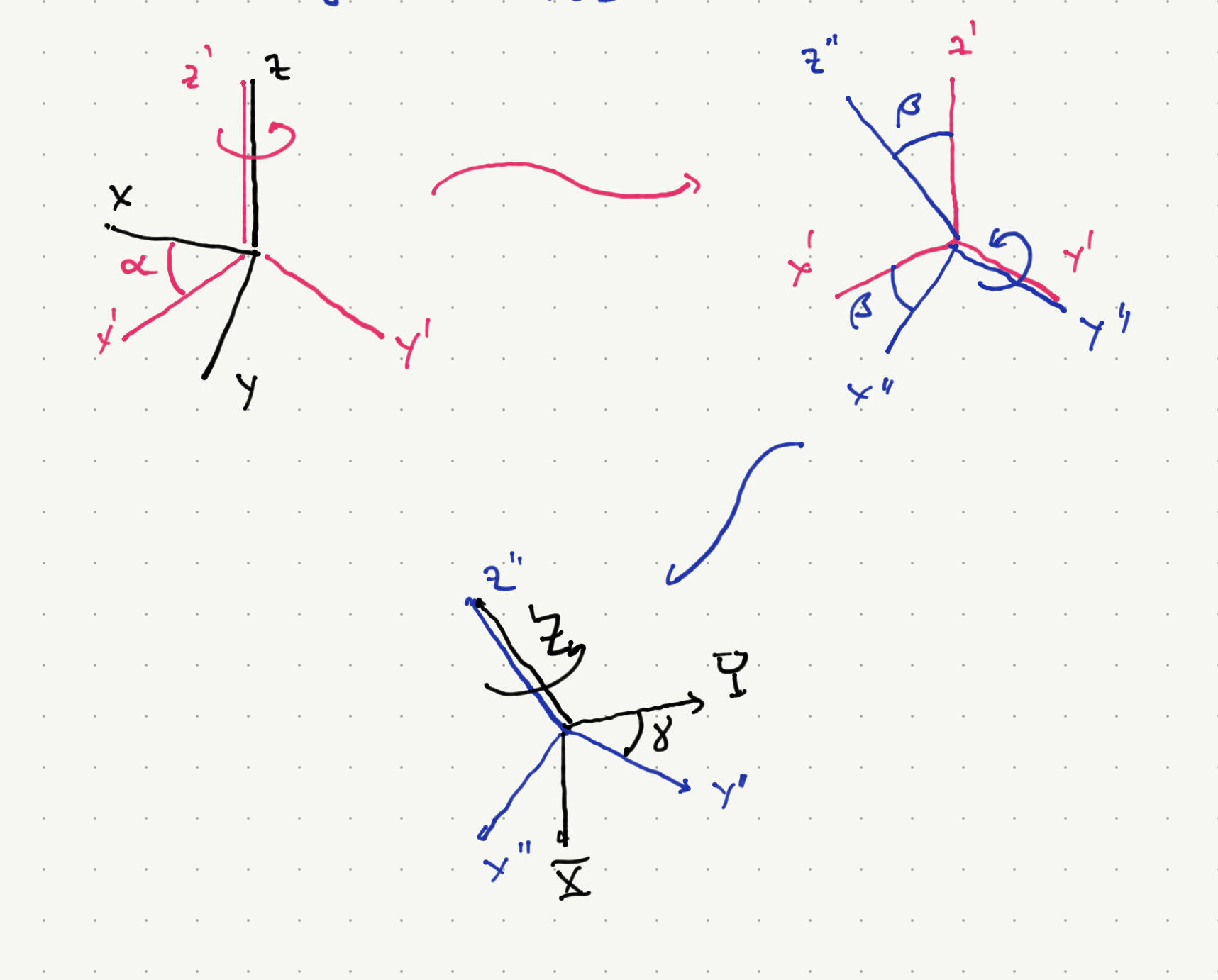
A general rotation can be described in terms of a transformation that rotates the axes attached to some rigid body, with respect to some coordinate axes initially aligned with the axes attached to that body. This can be done in the sequence described in the picture above; we can implement any rotation this way. First we rotate the frames around the \(z\) axis by an angle \(\alpha\). The resulting axes are labeled by \((x',y',z')\) where the \(z'\) acis and \(z\) axis still coincide. Then, we rotate by an angle \(\beta\) about the \(y\) axis which rotates the \(z'\) axis to the \(z''\) axis and the \(x'\) axis to the \(x''\) axis, keepingf the \(y'\) axis fixed (we can relabel it as \(y''\)). Note that at this point the \(y'/y''\) axis has not yet left the original \(x-y\) plane. Finally, we rotate the frame around the \(z''\) axis to new axes \(X,Y,Z\), with \(Z\) the same as \(Z''\). It should be clear that we can achieve any arbitrary rotation of the set of coordinate axes this way (maintaining their orthoginality and relative orientation).

We can describe this rotation as

\[R(\alpha,\beta,\gamma) = R({\hat Z},\gamma) R({\hat y'},\beta) R({\hat z},\alpha)\]

This expression holds for both the rotatoin matriceds and for the associate unibtary matrices in any representation, via the group homomorphism property.

The problem with this is that we would need to work out the rotation matrices (or their unitary representations) for the axes \(y',Z\). However, we can in fact rerite \(R\) in terms of rotations about the original axes. However, it is deducible from the pictures that we can write

(315)\[\begin{split}\begin{align} R({\hat Z},\gamma) & = R({\hat y}',\beta) R({\hat z},\gamma) R({\hat y}',-\beta)\\ R({\hat y}',\beta) & = R({\hat z},\alpha) R({\hat y},\beta) R({\hat z},-\alpha) \end{align}\end{split}\]

Using this,

\[\begin{split}\begin{align} R(\alpha,\beta,\gamma) & = R({\hat y}',\beta) R({\hat z}, \gamma) R({\hat y}',-\beta) R({\hat y'},\beta) R({\hat z},\alpha)\\ & = R({\hat y}',\beta) R({\hat z}, \gamma) R({\hat z},\alpha)\\ & = R({\hat z},\alpha) R({\hat y},\beta) R({\hat z},-\alpha) R({\hat z}, \gamma) R({\hat z},\alpha) \\ & = R({\hat z},\alpha) R({\hat y},\beta) R({\hat z},\gamma) R({\hat z}, -\alpha) R({\hat z},\alpha)\\ & = R({\hat z},\alpha) R({\hat y},\beta) R({\hat z},\gamma) \end{align}\end{split}\]

In the first line we used the first equation in conjugate_rot; in the second line we used the fact that \( R({\hat y}',-\beta) R({\hat y'},\beta) = {\bf 1}\); in the third line we used the second equation in conjugate_rot; in the fourth line we used the fact that successive rotations about \({\hat z}\) commute with each other; in the last equation we used \( R({\hat z}, -\alpha) R({\hat z},\alpha = {\bf 1}\).

In general, a given rotation \(R\) can be given a matrix representation in any irrep. We define

\[\bra{j,m'} U(R) \ket{j,m} = d^j_{m,m'}(R)\]

In the Euler angle representation,

\[U(R(\alpha,\beta,\gamma)) = e^{-i \alpha J_z/\hbar} e^{-i \beta J_y/\hbar} e^{-i \gamma J_z/\hbar}\]

Thus, we write

(316)\[d^j_{m',m}(\alpha,\beta,\gamma) = e^{-i m' \alpha - i m\gamma} \bra{j,m} e^{-i \beta J_y/\hbar} \ket{j,m}\]

Examples of irreps

Spin-\(0\)

This is the simplest/most trivial example; the corresponding irrep is one-dimensional. More generally there could be other degrees of freedom having nothing to do with angular momentum; we could imagine a situation where the angular momenbtum operator acts trivially on the whole Hilbert space so that every vector is a 1d irrep. More generally (in cases such as the hydrogen atom) we will find that there is a class of states which have \(j = 0\); inthe hydrogen atom (ignoring electron spin) these are the S-wave states.

Spin-\(\half\)

The first nontrivial example, and one we have studied many times. In the basis \(\ket{j,m} = \ket{\half,\pm \half}\), where \(\ket{\half,\half}\) is represented as \(\begin{pmatrix} 1 \\ 0 \end{pmatrix}\) and \(\ket{\half,-\half}\) is represented as \(\begin{pmatrix} 0 \\ 1 \end{pmatrix}\), we have

\[\begin{split}J_z = \frac{\hbar}{2} \begin{pmatrix} 1 & 0 \\ 0 & -1 \end{pmatrix} = \frac{\hbar}{2} \sigma_z\end{split}\]

Now using Equations (313), {eqlowering_op, we have

\[\begin{split}\begin{align} J_+ & = \hbar \begin{pmatrix} 0 & 1 \\ 0 & 0 \end{pmatrix} \\ J_- & = \hbar \begin{pmatrix} 0 & 0 \\ 1 & 0 \end{pmatrix} \end{align}\end{split}\]

Since \(J_{\pm} = J_x \pm i J_y\) we can solve for \(J_{x,y}\) to find

\[\begin{split}\begin{align} J_x & = \frac{J_+ + J_-}{2} = \frac{\hbar}{2} \begin{pmatrix} 0 & 1 \\ 1 & 0\end{pmatrix} = \frac{\hbar}{2} \sigma_x \\ J_y & = \frac{J_+ - J_-}{2i} = \frac{\hbar}{2} \begin{pmatrix} 0 & -i \\ i & 0\end{pmatrix} = \frac{\hbar}{2} \sigma_y \end{align}\end{split}\]

Note that these matrices are the same as appeared in the definition of \(SU(2)\). Finally \({\vec J}^2\) has eigenvalue \(\hbar^2 j(j+1) = \frac{3\hbar^2}{4}\).

A general rotation in the Euler angle representation can be calculated explicitly:

\[\begin{split}d^j_{m',m}(\alpha,\beta,\gamma) = \begin{pmatrix} e^{-i(\alpha + \gamma)/2} \cos\frac{\beta}{2} & - e^{-i(\alpha = \gamma)/2} \sin\frac{\beta}{2}\\ e^{i(\alpha - \gamma)/2}\sin \frac{\beta}{2} & e^{i(\alpha + \beta)/2} \cos\frac{\beta}{2} \end{pmatrix}\end{split}\]

Spin-\(1\)

The states \(\ket{1,m}\) with \(m \in \{-1,0,1\}\) form an orthonormal basis. Representing

\[\begin{split}\begin{align} \ket{1,1} & \to \begin{pmatrix} 1 \\ 0 \\ 0 \end{pmatrix}\\ \ket{1,0} & \to \begin{pmatrix} 0 \\ 1 \\ 0 \end{pmatrix}\\ \ket{1,-1} & \to \begin{pmatrix} 0 \\ 0 \\ -1 \end{pmatrix} \end{align}\end{split}\]

we can compute \(J_x\), \(J_{\pm}\), \(J_{x,y}\) as

\[\begin{split}\begin{align} J_z & = \hbar \begin{pmatrix} 1 & 0 & 0 \\ 0 & 0 & 0 \\ 0 & 0 & -1 \end{pmatrix}\\ J_+ & = \sqrt{2} \hbar \begin{pmatrix} 0 & 1 & 0 \\ 0 & 0 & 1 \\ 0 & 0 & 0 \end{pmatrix}\\ J_- & = \sqrt{2} \hbar \begin{pmatrix} 0 & 0 & 0 \\ 1 & 0 & 0 \\ 0 & 1 & 0 \end{pmatrix}\\ J_x & = \frac{\hbar}{\sqrt{2}} & = \begin{pmatrix} 0 & 1 & 0 \\ 1 & 0 & 1 \\ 0 & 1 & 0 \end{pmatrix}\\ J_y & = \frac{\hbar}{\sqrt{2}} \begin{pmatrix} 0 & -i & 0 \\ i & 0 & -i \\ 0 & i & o \end{pmatrix} \end{align}\end{split}\]

Unlike the case of spin-\(\half\), these are not the matrices that define infinitesimal rotations acting on real vectors in \(\CR^3\); we defined those in the previous section. In particular the component of \({\vec V}\) that is invariant under rotations about the \(z\) acis is \(V_z\). There are no real vectors which are eigenvectors of \(J_z\) with eigenvalue \(\pm 1\); the vectors which do have such behavior are complex, \(\frac{1}{\sqrt{2}} \begin{pmatrix} 1 \\ \pm i \\ 0 \end{pmatrix}\).